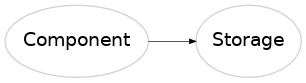
Storage class

Storage components store commodities and thus transfer commodities between time steps.

Storage class description:

class storage.Storage(esM, name, commodity, chargeRate=1, dischargeRate=1, chargeEfficiency=1, dischargeEfficiency=1, selfDischarge=0, cyclicLifetime=None, stateOfChargeMin=0, stateOfChargeMax=1, hasCapacityVariable=True, capacityVariableDomain='continuous', capacityPerPlantUnit=1, hasIsBuiltBinaryVariable=False, bigM=None, doPreciseTsaModeling=False, chargeOpRateMax=None, chargeOpRateFix=None, chargeTsaWeight=1, dischargeOpRateMax=None, dischargeOpRateFix=None, dischargeTsaWeight=1, isPeriodicalStorage=False, locationalEligibility=None, capacityMin=None, capacityMax=None, partLoadMin=None, sharedPotentialID=None, linkedQuantityID=None, capacityFix=None, commissioningMin=None, commissioningMax=None, commissioningFix=None, isBuiltFix=None, investPerCapacity=0, investIfBuilt=0, opexPerChargeOperation=0, opexPerDischargeOperation=0, opexPerCapacity=0, opexIfBuilt=0, interestRate=0.08, economicLifetime=10, technicalLifetime=None, floorTechnicalLifetime=True, socOffsetDown=-1, socOffsetUp=-1, stockCommissioning=None)[source]

A Storage component can store a commodity and thus transfers it between time steps.

__init__(esM, name, commodity, chargeRate=1, dischargeRate=1, chargeEfficiency=1, dischargeEfficiency=1, selfDischarge=0, cyclicLifetime=None, stateOfChargeMin=0, stateOfChargeMax=1, hasCapacityVariable=True, capacityVariableDomain='continuous', capacityPerPlantUnit=1, hasIsBuiltBinaryVariable=False, bigM=None, doPreciseTsaModeling=False, chargeOpRateMax=None, chargeOpRateFix=None, chargeTsaWeight=1, dischargeOpRateMax=None, dischargeOpRateFix=None, dischargeTsaWeight=1, isPeriodicalStorage=False, locationalEligibility=None, capacityMin=None, capacityMax=None, partLoadMin=None, sharedPotentialID=None, linkedQuantityID=None, capacityFix=None, commissioningMin=None, commissioningMax=None, commissioningFix=None, isBuiltFix=None, investPerCapacity=0, investIfBuilt=0, opexPerChargeOperation=0, opexPerDischargeOperation=0, opexPerCapacity=0, opexIfBuilt=0, interestRate=0.08, economicLifetime=10, technicalLifetime=None, floorTechnicalLifetime=True, socOffsetDown=-1, socOffsetUp=-1, stockCommissioning=None)[source]

Constructor for creating an Storage class instance. The Storage component specific input arguments are described below. The general component input arguments are described in the Component class.

Required arguments:

Parameters:: commodity (string) – to the component related commodity.

Default arguments:

Parameters:

chargeRate (0 <= float <=1) –
ratio of the maximum storage inflow (in commodityUnit/hour) to the storage capacity (in commodityUnit). Example:
- A hydrogen salt cavern which can store 133 GWh_H2_LHV can be charged 0.45 GWh_H2_LHV during one hour. The chargeRate thus equals 0.45/133 1/h.
* the default value is 1
dischargeRate (0 <= float <=1) –
ratio of the maximum storage outflow (in commodityUnit/hour) to the storage capacity (in commodityUnit). Example:
- A hydrogen salt cavern which can store 133 GWh_H2_LHV can be discharged 0.45 GWh_H2_LHV during one hour. The dischargeRate thus equals 0.45/133.
* the default value is 1
chargeEfficiency (0 <= float <=1) – defines the efficiency with which the storage can be charged (equals the percentage of the injected commodity that is transformed into stored commodity). Enter 0.98 for 98% etc.
* the default value is 1
dischargeEfficiency (0 <= float <=1) – defines the efficiency with which the storage can be discharged (equals the percentage of the withdrawn commodity that is transformed into stored commodity). Enter 0.98 for 98% etc.
* the default value is 1
selfDischarge (0 <= float <=1) – percentage of self-discharge from the storage during one hour
* the default value is 0
cyclicLifetime (None or positive float) – if specified, the total number of full cycle equivalents that are supported by the technology.
* the default value is None
stateOfChargeMin (0 <= float <=1) – threshold (percentage) that the state of charge can not drop under
* the default value is 0
stateOfChargeMax (0 <= float <=1) – threshold (percentage) that the state of charge can not exceed
* the default value is 1
doPreciseTsaModeling (boolean) – determines whether the state of charge is limited precisely (True) or with a simplified method (False). The error is small if the selfDischarge is small.
* the default value is False
chargeOpRateMax – if specified, indicates a maximum charging rate for each location and each time step, if required also for each investment period, by a positive float. If hasCapacityVariable is set to True, the values are given relative to the installed capacities (i.e. a value of 1 indicates a utilization of 100% of the capacity). If hasCapacityVariable is set to False, the values are given as absolute values in form of the commodityUnit, referring to the charged commodity (before multiplying the charging efficiency) during one time step.
* the default value is None
chargeOpRateFix – if specified, indicates a fixed charging rate for each location and each time step, if required also for each investment period, by a positive float. If hasCapacityVariable is set to True, the values are given relative to the installed capacities (i.e. a value of 1 indicates a utilization of 100% of the capacity). If hasCapacityVariable is set to False, the values are given as absolute values in form of the commodityUnit, referring to the charged commodity (before multiplying the charging efficiency) during one time step.
* the default value is None
chargeTsaWeight (positive (>= 0) float) – weight with which the chargeOpRate (max/fix) time series of the component should be considered when applying time series aggregation.
* the default value is 1
dischargeOpRateMax – if specified, indicates a maximum discharging rate for each location and each time step, if required also for each investment period, by a positive float. If hasCapacityVariable is set to True, the values are given relative to the installed capacities (i.e. a value of 1 indicates a utilization of 100% of the capacity). If hasCapacityVariable is set to False, the values are given as absolute values in form of the commodityUnit, referring to the discharged commodity (after multiplying the discharging efficiency) during one time step.
* the default value is None
dischargeOpRateFix – if specified, indicates a fixed discharging rate for each location and each time step, if required also for each investment period, by a positive float. If hasCapacityVariable is set to True, the values are given relative to the installed capacities (i.e. a value of 1 indicates a utilization of 100% of the capacity). If hasCapacityVariable is set to False, the values are given as absolute values in form of the commodityUnit, referring to the charged commodity (after multiplying the discharging efficiency) during one time step.
* the default value is None
dischargeTsaWeight (positive (>= 0) float) – weight with which the dischargeOpRate (max/fix) time series of the component should be considered when applying time series aggregation.
* the default value is 1
isPeriodicalStorage (boolean) – indicates if the state of charge of the storage has to be at the same value after the end of each period. This is especially relevant when using daily periods where short term storage can be restrained to daily cycles. Benefits the run time of the model.
* the default value is False
opexPerChargeOperation (positive (>=0) float or Pandas Series with positive (>=0) values or dict of positive (>=0) float or Pandas Series with positive (>=0) values per investment period. The indices of the series have to equal the in the energy system model specified locations.) – describes the cost for one unit of the charge operation. The cost which is directly proportional to the charge operation of the component is obtained by multiplying the opexPerChargeOperation parameter with the annual sum of the operational time series of the components. The opexPerChargeOperation can either be given as a float or a Pandas Series with location specific values or a dictionary per investment period with one of the two previous options. The cost unit in which the parameter is given has to match the one specified in the energy system model (e.g. Euro, Dollar, 1e6 Euro).
* the default value is 0
opexPerDischargeOperation – describes the cost for one unit of the discharge operation. The cost which is directly proportional to the discharge operation of the component is obtained by multiplying the opexPerDischargeOperation parameter with the annual sum of the operational time series of the components. The opexPerDischargeOperation can either be given as a float or a Pandas Series with location specific values or a dictionary per investment period with one of the two previous options. The cost unit in which the parameter is given has to match the one specified in the energy system model (e.g. Euro, Dollar, 1e6 Euro).
* the default value is 0
socOffsetDown (float) – determines whether the state of charge at the end of a period p has to be equal to the one at the beginning of a period p+1 (socOffsetDown=-1) or if it can be smaller at the beginning of p+1 (socOffsetDown>=0). In the latter case, the product of the parameter socOffsetDown and the actual soc offset is used as a penalty factor in the objective function.
* the default value is -1
socOffsetUp (float) – determines whether the state of charge at the end of a period p has to be equal to the one at the beginning of a period p+1 (socOffsetUp=-1) or if it can be larger at the beginning of p+1 (socOffsetUp>=0). In the latter case, the product of the parameter socOffsetUp and the actual soc offset is used as a penalty factor in the objective function.
* the default value is -1

setTimeSeriesData(hasTSA)[source]

Function for setting the maximum operation rate and fixed operation rate for charging and discharging depending on whether a time series analysis is requested or not.

Parameters:: hasTSA (boolean) – states whether a time series aggregation is requested (True) or not (False).

getDataForTimeSeriesAggregation(ip)[source]

Function for getting the required data if a time series aggregation is requested.

Parameters:: ip (int) – investment period of transformation path analysis.

setAggregatedTimeSeriesData(data, ip)[source]

Function for determining the aggregated maximum rate and the aggregated fixed operation rate for charging and discharging.

Parameters:

data (Pandas DataFrame) – Pandas DataFrame with the clustered time series data of the source component
ip (int) – investment period of transformation path analysis.

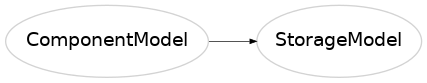
checkProcessedDataSets()[source]: Check processed time series data after applying time series aggregation. If all entries of dictionary are None the parameter itself is set to None.

Inheritance diagram:

StorageModel class description:

class storage.StorageModel[source]

A StorageModel class instance will be instantly created if a Storage class instance is initialized. It is used for the declaration of the sets, variables and constraints which are valid for the Storage class instance. These declarations are necessary for the modeling and optimization of the energy system model. The StorageModel class inherits from the ComponentModel class.

declareSets(esM, pyM)[source]

Declare sets: design variable sets, operation variable set, operation mode sets.

Parameters:

esM (esM - EnergySystemModel class instance) – EnergySystemModel instance representing the energy system in which the component should be modeled.
pyM (pyomo ConcreteModel) – pyomo ConcreteModel which stores the mathematical formulation of the model.

declareVariables(esM, pyM, relaxIsBuiltBinary, relevanceThreshold)[source]

Declare design and operation variables.

Parameters:

esM (esM - EnergySystemModel class instance) – EnergySystemModel instance representing the energy system in which the component should be modeled.
pyM (pyomo ConcreteModel) – pyomo ConcreteModel which stores the mathematical formulation of the model.
relaxIsBuiltBinary – states if the optimization problem should be solved as a relaxed LP to get the lower bound of the problem.
* the default value is False
relevanceThreshold (float (>=0) or None) – Force operation parameters to be 0 if values are below the relevance threshold.
* the default value is None

connectSOCs(pyM, esM)[source]

Declare the constraint for connecting the state of charge with the charge and discharge operation: the change in the state of charge between two points in time has to match the values of charging and discharging (considering the efficiencies of these processes) within the time step in between minus the self-discharge of the storage.

$\begin{eqnarray*} SoC^{comp}_{loc,ip,p,t+1} - \left( SoC^{comp}_{loc,ip,p,t} \left( 1 - \eta^{self-discharge} \right)^{\frac{\tau^{hours}}{h}} + op^{comp,charge}_{loc,ip,p,t} \eta^{charge} - op^{comp,discharge}_{loc,ip,p,t} / \eta^{discharge} \right) = 0 \end{eqnarray*}$

Parameters:

pyM (pyomo ConcreteModel) – pyomo ConcreteModel which stores the mathematical formulation of the model.
esM (esM - EnergySystemModel class instance) – EnergySystemModel instance representing the energy system in which the component should be modeled.

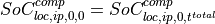
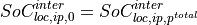
cyclicState(pyM, esM)[source]

Declare the constraint for connecting the states of charge: the state of charge at the beginning of a period has to be the same as the state of charge in the end of that period.

with full temporal resolution

$SoC^{comp}_{loc,ip,0,0} = SoC^{comp}_{loc,ip,0,t^{total}}$

with time series aggregation:

$SoC^{inter}_{loc,ip,0} = SoC^{inter}_{loc,ip,p^{total}}$

Parameters:

pyM (pyomo ConcreteModel) – pyomo ConcreteModel which stores the mathematical formulation of the model.
esM (esM - EnergySystemModel class instance) – EnergySystemModel instance representing the energy system in which the component should be modeled.

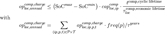
cyclicLifetime(pyM, esM)[source]

Declare the constraint for limiting the number of full cycle equivalents to stay below cyclic lifetime.

$\begin{eqnarray*} & & op^{comp,charge}_{loc,annual} \leq \left( \text{SoC}^{max} - \text{SoC}^{min} \right) \cdot cap^{comp}_{loc,ip} \cdot \frac{t^{ \text{comp,cyclic lifetime}}}{\tau^{ \text{comp,economic lifetime}}_{loc}} \\ \text{with} \\ & & op^{comp,charge}_{loc,annual} = \sum_{(ip,p,t) \in \mathcal{P} \times \mathcal{T}} op^{comp,charge}_{loc,ip,p,t} \cdot freq(p) / \tau^{years} \end{eqnarray*}$

Parameters:

pyM (pyomo ConcreteModel) – pyomo ConcreteModel which stores the mathematical formulation of the model.
esM (esM - EnergySystemModel class instance) – EnergySystemModel instance representing the energy system in which the component should be modeled.

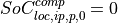
connectInterPeriodSOC(pyM, esM)[source]

Declare the constraint that the state of charge at the end of each period has to be equivalent to the state of charge of the period before it (minus its self discharge) plus the change in the state of charge which happened during the typical period which was assigned to that period.

$\begin{eqnarray*} SoC^{inter}_{loc,ip,p+1} - SoC^{inter}_{loc,ip,p} \cdot \left( 1 - \eta^{self-discharge} \right)^{\frac{t^{\text{per period}} \cdot \tau^{hours}}{h}} \ SoC^{comp}_{loc,ip,map(p),t^{\text{per period}}} = 0 \end{eqnarray*}$

Parameters:

pyM (pyomo ConcreteModel) – pyomo ConcreteModel which stores the mathematical formulation of the model.
esM (esM - EnergySystemModel class instance) – EnergySystemModel instance representing the energy system in which the component should be modeled.

intraSOCstart(pyM, esM)[source]

Declare the constraint that the (virtual) state of charge at the beginning of a typical period is zero.

$SoC^{comp}_{loc,ip,p,0} = 0$

Parameters:

pyM (pyomo ConcreteModel) – pyomo ConcreteModel which stores the mathematical formulation of the model.
esM (esM - EnergySystemModel class instance) – EnergySystemModel instance representing the energy system in which the component should be modeled.

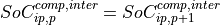
equalInterSOC(pyM, esM)[source]

Declare the constraint that, if periodic storage is selected, the states of charge between periods have the same value.

$SoC^{comp,inter}_{ip,p} = SoC^{comp,inter}_{ip,p+1}$

Parameters:

pyM (pyomo ConcreteModel) – pyomo ConcreteModel which stores the mathematical formulation of the model.
esM (esM - EnergySystemModel class instance) – EnergySystemModel instance representing the energy system in which the component should be modeled.

minSOC(pyM)[source]

Declare the constraint that the state of charge [commodityUnit*h] has to be larger than the installed capacity [commodityUnit*h] multiplied with the relative minimum state of charge.

$SoC^{comp,min} \cdot cap^{comp}_{loc,ip} \leq SoC^{comp}_{loc,ip,0,t}$

Parameters:: pyM (pyomo ConcreteModel) – pyomo ConcreteModel which stores the mathematical formulation of the model.

limitSOCwithSimpleTsa(pyM, esM)[source]

Simplified version of the state of charge limitation control. The error compared to the precise version is small in cases of small selfDischarge.

$\begin{eqnarray*} & & \underline{SoC}^{comp,sup}_{loc,ip,p,t} \geq \text{SoC}^{min} \cdot cap^{comp}_{loc,ip} \\ & & \overline{SoC}^{comp,sup}_{loc,ip,p,t} \leq \text{SoC}^{max} \cdot cap^{comp}_{loc,ip} \\ \text{with } \\ & & \underline{SoC}^{comp,sup}_{loc,ip,p,t} = SoC^{inter}_{loc,ip,p} \cdot (1 - \eta^{\text{self-discharge}})^{\frac{t^{\text{per period}} \cdot \tau^{hours}}{h}}+ SoC^{min}_{loc,ip,map(p)} \\ & &\overline{SoC}^{comp,sup}_{loc,ip,p,t} = SoC^{inter}_{loc,ip,p} + SoC^{max}_{loc,ip,map(p)} \end{eqnarray*}$

Parameters:

pyM (pyomo ConcreteModel) – pyomo ConcreteModel which stores the mathematical formulation of the model.
esM (esM - EnergySystemModel class instance) – EnergySystemModel instance representing the energy system in which the component should be modeled.

operationModeSOC(pyM, esM)[source]

Declare the constraint that the state of charge [commodityUnit*h] is limited by the installed capacity [commodityUnit*h] and the relative maximum state of charge [-].

$SoC^{comp}_{loc,ip,0,t} \leq \text{SoC}^{comp,max} \cdot cap^{comp}_{loc,ip}$

Parameters:

pyM (pyomo ConcreteModel) – pyomo ConcreteModel which stores the mathematical formulation of the model.
esM (esM - EnergySystemModel class instance) – EnergySystemModel instance representing the energy system in which the component should be modeled.

operationModeSOCwithTSA(pyM, esM)[source]

Declare the constraint that the state of charge [commodityUnit*h] is limited by the installed capacity # [commodityUnit*h] and the relative maximum state of charge [-].

$SoC^{inter}_{loc,ip,p} \cdot (1 - \eta^{\text{self-discharge}})^{\frac{t \cdot \tau^{hours}}{h}} + SoC^{comp}_{loc,ip,map(p),t} \leq \text{SoC}^{max} \cdot cap^{comp}_{loc,ip}$

Parameters:

pyM (pyomo ConcreteModel) – pyomo ConcreteModel which stores the mathematical formulation of the model.
esM (esM - EnergySystemModel class instance) – EnergySystemModel instance representing the energy system in which the component should be modeled.

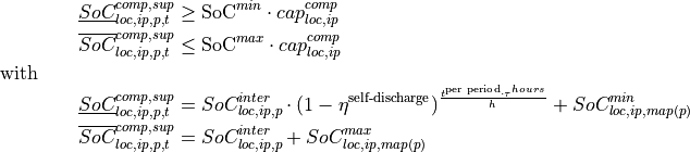
minSOCwithTSAprecise(pyM, esM)[source]

Declare the constraint that the state of charge [commodityUnit*h] at each time step cannot be smaller than the installed capacity [commodityUnit*h] multiplied with the relative minimum state of charge [-].

$\text{SoC}^{min} \cdot cap^{comp}_{loc,ip} \leq SoC^{inter}_{loc,ip,p} \cdot (1 - \eta^{\text{self-discharge}})^{\frac{t \cdot \tau^{hours}}{h}} + SoC^{comp}_{loc,ip,map(p),t}$

Parameters:

pyM (pyomo ConcreteModel) – pyomo ConcreteModel which stores the mathematical formulation of the model.
esM (esM - EnergySystemModel class instance) – EnergySystemModel instance representing the energy system in which the component should be modeled.

declareComponentConstraints(esM, pyM)[source]

Declare time independent and dependent constraints.

Parameters:

esM (esM - EnergySystemModel class instance) – EnergySystemModel instance representing the energy system in which the component should be modeled.
pyM (pyomo ConcreteModel) – pyomo ConcreteModel which stores the mathematical formulation of the model.

hasOpVariablesForLocationCommodity(esM, loc, commod)[source]

Check if operation variables exist in the modeling class at a location which are connected to a commodity.

Parameters:

esM (esM - EnergySystemModel class instance) – EnergySystemModel instance representing the energy system in which the component should be modeled.
loc (string) – Name of the regarded location (locations are defined in the EnergySystemModel instance)
commod – Name of the regarded commodity (commodities are defined in the EnergySystemModel instance)
commod – string

getCommodityBalanceContribution(pyM, commod, loc, ip, p, t)[source]: Get contribution to a commodity balance.

$\text{C}^{comp,comm}_{loc,ip,p,t} = op^{comp,discharge}_{loc,ip,p,t} - op^{comp,charge}_{loc,ip,p,t}$

getObjectiveFunctionContribution(esM, pyM)[source]

Get contribution to the objective function.

Parameters:

esM (esM - EnergySystemModel class instance) – EnergySystemModel instance representing the energy system in which the component should be modeled.
pyM (pyomo ConcreteModel) – pyomo ConcreteModel which stores the mathematical formulation of the model.

setOptimalValues(esM, pyM)[source]

Set the optimal values of the components.

Parameters:

esM (esM - EnergySystemModel class instance) – EnergySystemModel instance representing the energy system in which the component should be modeled.
pyM (pyomo ConcreteModel) – pyomo ConcreteModel which stores the mathematical formulation of the model.

getOptimalValues(name='all', ip=0)[source]

Return optimal values of the components.

Parameters:

name –

name of the variables of which the optimal values should be returned:

’capacityVariables’,
’isBuiltVariables’,
’chargeOperationVariablesOptimum’,
’dischargeOperationVariablesOptimum’,
’stateOfChargeOperationVariablesOptimum’,
’all’ or another input: all variables are returned.

For optimizations with several years also following values should be returned: * ‘_operationVariablesOptimum’ * ‘_decommissioningVariablesOptimum’

* the default value is ‘all’ :type name: string

Parameters:: ip (int) – investment period
* the default value is 0
Returns:: a dictionary with the optimal values of the components
Return type:: dict

Inheritance diagram: