EnergySystemModel class
A description of the class is given below.
Class description:
- class energySystemModel.EnergySystemModel(locations, commodities, commodityUnitsDict, numberOfTimeSteps=8760, hoursPerTimeStep=1, startYear=0, numberOfInvestmentPeriods=1, investmentPeriodInterval=1, stochasticModel=False, costUnit='1e9 Euro', lengthUnit='km', verboseLogLevel=0, balanceLimit=None, pathwayBalanceLimit=None, annuityPerpetuity=False)[source]
EnergySystemModel class
The functionality provided by the EnergySystemModel class is fourfold:
With it, the basic structure (spatial and temporal resolution, considered commodities) of the investigated energy system is defined.
It serves as a container for all components investigated in the energy system model. These components, namely sources and sinks, conversion options, storage options, and transmission options (in the core module), can be added to an EnergySystemModel instance.
It provides the core functionality of modeling and optimizing the energy system based on the specified structure and components on the one hand and of specified simulation parameters on the other hand.
It stores optimization results which can then be post-processed with other modules.
The parameters which are stored in an instance of the class refer to:
the modeled spatial representation of the energy system (locations, lengthUnit)
the modeled temporal representation of the energy system (totalTimeSteps, hoursPerTimeStep, startYear, numberOfInvementPeriods, investmentPeriodInterval, periods, periodsOrder, periodsOccurrences, timeStepsPerPeriod, interPeriodTimeSteps, isTimeSeriesDataClustered, typicalPeriods, tsaInstance, timeUnit)
the considered commodities in the energy system (commodities, commodityUnitsDict)
the considered components in the energy system (componentNames, componentModelingDict, costUnit)
optimization related parameters (pyM, solverSpecs)
The parameters are first set when a class instance is initiated. The parameters which are related to the components (e.g. componentNames) are complemented by adding the components to the class instance.
Instances of this class provide functions for
adding components and their respective modeling classes (add)
clustering the time series data of all added components using the time series aggregation package tsam, cf. https://github.com/FZJ-IEK3-VSA/tsam (cluster)
optimizing the specified energy system (optimize), for which a pyomo concrete model instance is built and filled with
basic time sets,
sets, variables and constraints contributed by the component modeling classes,
basic, component overreaching constraints, and
an objective function.
The pyomo instance is then optimized by a specified solver. The optimization results are processed once available.
getting components and their attributes (getComponent, getCompAttr, getOptimizationSummary)
- __init__(locations, commodities, commodityUnitsDict, numberOfTimeSteps=8760, hoursPerTimeStep=1, startYear=0, numberOfInvestmentPeriods=1, investmentPeriodInterval=1, stochasticModel=False, costUnit='1e9 Euro', lengthUnit='km', verboseLogLevel=0, balanceLimit=None, pathwayBalanceLimit=None, annuityPerpetuity=False)[source]
Constructor for creating an EnergySystemModel class instance
Required arguments:
- Parameters:
locations (set of strings) – locations considered in the energy system
commodities (set of strings) – commodities considered in the energy system
commodityUnitsDict (dictionary of strings) –
dictionary which assigns each commodity a quantitative unit per time (e.g. GW_el, GW_H2, Mio.t_CO2/h). The dictionary is used for results output.
Note
Note for advanced users: the scale of these units can influence the numerical stability of the optimization solver, cf. http://files.gurobi.com/Numerics.pdf where a reasonable range of model coefficients is suggested.
Default arguments:
- Parameters:
numberOfTimeSteps – number of time steps considered when modeling the energy system (for each time step, or each representative time step, variables and constraints are constituted). Together with the hoursPerTimeStep, the total number of hours considered can be derived. The total number of hours is again used for scaling the arising costs to the arising total annual costs (TAC) which are minimized during optimization.
* the default value is 8760.hoursPerTimeStep (strictly positive float) – hours per time step
* the default value is 1numberOfInvestmentPeriods (strictly positive integer) – number of investment periods of transformation path analysis, e.g. for a transformation pathway from 2020 to 2030 with the years 2020, 2025, 2030, the numberOfInvestmentPeriods is 3
* the default value is 1investmentPeriodInterval (strictly positive integer) – interval between the investment of transformation path analysis, e.g. for a transformation pathway from 2020 to 2030 with the years 2020, 2025, 2030, the investmentPeriodInterval is 5
* the default value is 1startYear (integer) – year name of first investment period, e.g. for a transformation pathway from 2020 to 2030 with the years 2020, 2025, 2030, the startYear is 2020
* the default value is 0stochasticModel – defines whether to set up a stochastic optimization. The goal of the stochastic optimization is to find a more robust energy system by considering different requirements to find a single energy system design (e.g. various weather years or demand forecasts). These requirements are represented in different investment periods of the model. In contrast to the classical perfect foresight optimization the investment periods do not represent steps of a tranformation pathway but possible boundary conditions for the energy system, which need to be considered for the system design and operation
* the default value is FalsecostUnit (string) –
cost unit of all cost related values in the energy system. This argument sets the unit of all cost parameters which are given as an input to the EnergySystemModel instance (e.g. for the invest per capacity or the cost per operation).
Note
Note for advanced users: the scale of this unit can influence the numerical stability of the optimization solver, cf. http://files.gurobi.com/Numerics.pdf where a reasonable range of model coefficients is suggested.
* the default value is ‘10^9 Euro’ (billion euros), which can be a suitable scale for national energy systems.lengthUnit (string) –
length unit for all length-related values in the energy system.
Note
Note for advanced users: the scale of this unit can influence the numerical stability of the optimization solver, cf. http://files.gurobi.com/Numerics.pdf where a reasonable range of model coefficients is suggested.
* the default value is ‘km’ (kilometers).verboseLogLevel (integer (0, 1 or 2)) –
defines how verbose the console logging is:
0: general model logging, warnings and optimization solver logging are displayed.
1: warnings are displayed.
2: no general model logging or warnings are displayed, the optimization solver logging is set to a minimum.
Note
if required, the optimization solver logging can be separately enabled in the optimizationSpecs of the optimize function.
* the default value is 0balanceLimit –
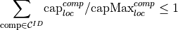
defines the balanceLimit constraint (various different balanceLimitIDs possible) for specific regions or the whole model and optional also per investment period. The balancelimitID can be assigned to various components of e.g. SourceSinkModel or TransmissionModel to limit the balance of production, consumption and im/export.
Regional dependency: The balanceLimit is defined as a pd.DataFrame. Each row contains an individual balanceLimitID as index, the corresponding regional scope as columns and the values as data. The regional scope can be set for a region with the matching region name as column name or “Total” as colum name for setting for the entire system. Example: - per region: pd.DataFrame(columns=[“Region1”], index=[“electricity”], data=[1000]) - per region and per system: pd.DataFrame(columns=[“Region1”,”Total”], index=[“electricity”], data=[1000,2000])
Temporal dependency: If the balanceLimit is passed as a dict with the described pd.DataFrames as values it is considered per investment period. Values are always given in the unit of the esM commodities unit.
Optional: A column named ‘lowerBound’ can be passed to specify if the limit is an upper or lower bound. By default an upperBound is considered (‘lowerBound’=False). However, multiple cases can be considered:
Sources:
a) LowerBound=False: UpperBound for commodity from SourceComponent (Define positive value in balanceLimit). Example: Limit CO2-Emission
b) LowerBound=True: LowerBound for commodity from SourceComponent (Define positive value in balanceLimit). Example: Require minimum production from renewables.
Sinks:
a) LowerBound=False: UpperBound in a mathematical sense for commodity from SinkComponent (Logically minimum limit for negative values, define negative value in balanceLimit). Example: Minimum export/consumption of hydrogen.
b) LowerBound=True: LowerBound in a mathematical sense for commodity from SourceComponent (Logically maximum limit for negative values, define negative value in balanceLimit). Example: Define upper limit for Carbon Capture & Storage.
Note
If bounds for sinks shall be specified (e.g. min. export, max. sink volume), values must be defined as negative.
* the default value is NonepathwayBalanceLimit (None or pd.DataFrame) – the pathway balance limit defines commodity balance (lower or upper bound) for the pathway. The structure is similar to the balanceLimit, however does without the temporal dependency per investment period. Examples: CO2 budget for the entire transformation pathway
* the default value is NoneannuityPerpetuity –
if set to True, it is assumed that the design and operation of the last investment period will be maintained forever. Therefore, the cost contribution of each component’s last investment period is divided by the component’s interest rate to account for perpetuity costs.
To enable annuity perpetuity the interest rate of every component must be greater than 0.
* the default value is False
- Type:
annuityPerpetuity: bool
- add(component)[source]
Function for adding a component and, if required, its respective modeling class to the EnergySystemModel instance. The added component has to inherit from the FINE class Component.
- Parameters:
component (An object which inherits from the FINE Component class) – the component to be added
- removeComponent(componentName, track=False)[source]
Function which removes a component from the energy system.
- Parameters:
componentName (string) – name of the component that should be removed
track (boolean) – specifies if the removed components should be tracked or not
* the default value is False
- Returns:
dictionary with the removed componentName and component instance if track is set to True else None.
- Return type:
dict or None
- getComponent(componentName)[source]
Function which returns a component of the energy system.
- Parameters:
componentName (string) – name of the component that should be returned
- Returns:
the component which has the name componentName
- Return type:
- updateComponent(componentName, updateAttrs)[source]
Overwrite selected attributes of an existing esM component with new values.
Note
Be aware of the fact that some attributes are filled automatically while initializing a component. E.g., if you want to change attributes like economic lifetime, there might occur the error that the new value does not match with the technical lifetime of the component. Additionally: You cannot change the name of an existing component by using this function. If you do so, you will not update the component but create a new one with the new name. The old component will still exist.
- getComponentAttribute(componentName, attributeName)[source]
Function which returns an attribute of a component considered in the energy system.
- Parameters:
componentName (string) – name of the component from which the attribute should be obtained
attributeName (string) – name of the attribute that should be returned
- Returns:
the attribute specified by the attributeName of the component with the name componentName
- Return type:
depends on the specified attribute
- getOptimizationSummary(modelingClass, ip=0, outputLevel=0)[source]
Function which returns the optimization summary (design variables, aggregated operation variables, objective contributions) of a modeling class.
- Parameters:
modelingClass (string) – name of the modeling class from which the optimization summary should be obtained
outputLevel (integer (0, 1 or 2)) –
states the level of detail of the output summary:
0: full optimization summary is returned
1: full optimization summary is returned but rows in which all values are NaN (not a number) are dropped
2: full optimization summary is returned but rows in which all values are NaN or 0 are dropped
* the default value is 0
- Returns:
the optimization summary of the requested modeling class
- Return type:
pandas DataFrame
- aggregateSpatially(shapefile, grouping_mode='parameter_based', n_groups=3, distance_threshold=None, aggregatedResultsPath=None, **kwargs)[source]
Spatially clusters the data of all components considered in the Energy System Model (esM) instance and returns a new esM instance with the aggregated data.
- Parameters:
shapefile (string, GeoDataFrame) – Either the path to the shapefile or the read-in shapefile
Default arguments:
- Parameters:
grouping_mode (string, Options: 'string_based', 'distance_based', 'parameter_based') – Defines how to spatially group the regions. Refer to grouping.py for more information.
* the default value is ‘parameter_based’n_groups (strictly positive integer, None) – The number of region groups to be formed from the original region set. This parameter is irrelevant if grouping_mode is ‘string_based’.
* the default value is 3distance_threshold (float) – The distance threshold at or above which regions will not be aggregated into one.
* the default value is None. If not None, n_groups must be NoneaggregatedResultsPath (string, None) – Indicates path to which the aggregated results should be saved. If None, results are not saved.
* the default value is None
Additional keyword arguments that can be passed via kwargs:
- Parameters:
geom_col_name (string) – The geometry column name in shapefile
* the default value is ‘geometry’geom_id_col_name (string) – The colum in shapefile consisting geom IDs
* the default value is ‘index’separator (string) – Relevant only if grouping_mode is ‘string_based’. The character or string in the region IDs that defines where the ID should be split. E.g.: region IDs -> [‘01_es’, ‘02_es’] and separator=’_’, then IDs are split at _ and the last part (‘es’) is taken as the group ID
* the default value is Noneposition (integer/tuple) –
Relevant only if grouping_mode is ‘string_based’. Used to define the position(s) of the region IDs where the split should happen. An int i would mean the part from 0 to i is taken as the group ID. A tuple (i,j) would mean the part i to j is taken at the group ID.
Note
either separator or position must be passed in order to perform string_based_grouping
* the default value is Noneweights (dictionary) –
Relevant only if grouping_mode is ‘parameter_based’. Through the weights dictionary, one can assign weights to variable-component pairs. When calculating distance corresponding to each variable-component pair, these specified weights are considered, otherwise taken as 1.
It must be in one of the formats:
If you want to specify weights for particular variables and particular corresponding components:
{ ‘components’ : Dict[<component_name>, <weight>}], ‘variables’ : List[<variable_name>] }
If you want to specify weights for particular variables, but all corresponding components:
{ ‘components’ : {‘all’ : <weight>}, ‘variables’ : List[<variable_name>] }
If you want to specify weights for all variables, but particular corresponding components:
{ ‘components’ : Dict[<component_name>, <weight>}], ‘variables’ : ‘all’ }
<weight> can be of type integer/float
* the default value is Noneaggregation_method (string, Options: 'kmedoids_contiguity', 'hierarchical') –
Relevant only if grouping_mode is ‘parameter_based’. The clustering method that should be used to group the regions. Options:
- ’kmedoids_contiguity’:
kmedoids clustering with added contiguity constraint. Refer to TSAM docs for more info: https://github.com/FZJ-IEK3-VSA/tsam/blob/master/tsam/utils/k_medoids_contiguity.py
- ’hierarchical’:
sklearn’s agglomerative clustering with complete linkage, with a connetivity matrix to ensure contiguity. Refer to Sklearn docs for more info: https://scikit-learn.org/stable/modules/generated/sklearn.cluster.AgglomerativeClustering.html
* the default value is ‘kmedoids_contiguity’solver (string, Options: 'gurobi', 'glpk') – Relevant only if grouping_mode is ‘parameter_based’ and aggregation_method is ‘kmedoids_contiguity’ The optimization solver to be chosen.
* the default value is ‘gurobi’aggregation_function_dict (dictionary) –
Contains information regarding the mode of aggregation for each individual variable.
Possibilities: mean, weighted mean, sum, bool (boolean OR).
Format of the dictionary
{<variable_name>: (<mode_of_aggregation>, <weights>), <variable_name>: (<mode_of_aggregation>, None)}.
<weights> is required only if <mode_of_aggregation> is ‘weighted mean’. The name of the variable that should act as weights should be provided. Can be None otherwise.
A default dictionary is considered with the following corresponding modes. If aggregation_function_dict is passed, this default dictionary is updated.
{“operationRateMax”: (“weighted mean”, “capacityMax”),”operationRateFix”: (“sum”, None),”processedLocationalEligibility”: (“bool”, None),”capacityMax”: (“sum”, None),”investPerCapacity”: (“mean”, None),”investIfBuilt”: (“bool”, None),”opexPerOperation”: (“mean”, None),”opexPerCapacity”: (“mean”, None),”opexIfBuilt”: (“bool”, None),”interestRate”: (“mean”, None),”economicLifetime”: (“mean”, None),”capacityFix”: (“sum”, None),”losses”: (“mean”, None),”distances”: (“mean”, None),”commodityCost”: (“mean”, None),”commodityRevenue”: (“mean”, None),”opexPerChargeOperation”: (“mean”, None),”opexPerDischargeOperation”: (“mean”, None),”QPcostScale”: (“sum”, None),”technicalLifetime”: (“mean”, None)}aggregated_shp_name (string) – Name to be given to the saved shapefiles after aggregation
* the default value is ‘aggregated_regions’crs (integer) – Coordinate reference system (crs) in which to save the shapefiles
* the default value is 3035crs – Coordinate reference system (crs) in which to save the shapefiles
* the default value is 3035aggregated_xr_filename (string) – Name to be given to the saved netCDF file containing aggregated esM data
* the default value is ‘aggregated_xr_dataset.nc’
- Returns:
Aggregated esM instance
- aggregateTemporally(numberOfTypicalPeriods=40, numberOfTimeStepsPerPeriod=24, segmentation=True, numberOfSegmentsPerPeriod=12, clusterMethod='hierarchical', representationMethod='durationRepresentation', sortValues=False, storeTSAinstance=False, rescaleClusterPeriods=False, **kwargs)[source]
Temporally cluster the time series data of all components considered in the EnergySystemModel instance and then stores the clustered data in the respective components. For this, the time series data is broken down into an ordered sequence of periods (e.g. 365 days) and to each period a typical period (e.g. 7 typical days with 24 hours) is assigned. Moreover, the time steps within the periods can further be clustered to bigger time steps with an irregular duration using the segmentation option. For the clustering itself, the tsam package is used (cf. https://github.com/FZJ-IEK3-VSA/tsam). Additional keyword arguments for the TimeSeriesAggregation instance can be added (facilitated by kwargs). As an example: it might be useful to add extreme periods to the clustered typical periods.
Note
The segmentation option can be freely combined with all subclasses. However, an irregular time step length is not meaningful for the minimumDownTime and minimumUpTime in the conversionDynamic module, because the time would be different for each segment.
Default arguments:
- Parameters:
numberOfTypicalPeriods (strictly positive integer) –
states the number of typical periods into which the time series data should be clustered. The number of time steps per period must be an integer multiple of the total number of considered time steps in the energy system.
Note
Please refer to the tsam package documentation of the parameter noTypicalPeriods for more information.
* the default value is 7numberOfTimeStepsPerPeriod (strictly positive integer) – states the number of time steps per period
* the default value is 24segmentation (boolean) – states whether the typical periods should be further segmented to fewer time steps
* the default value is FalsenumberOfSegmentsPerPeriod (strictly positive integer) – states the number of segments per period
* the default value is 24clusterMethod (string) –
states the method which is used in the tsam package for clustering the time series data. Options are for example ‘averaging’, ‘k_means’, ‘exact k_medoid’ or ‘hierarchical’.
Note
Please refer to the tsam package documentation of the parameter clusterMethod for more information.
* the default value is ‘hierarchical’representationMethod (string) –
Chosen representation. If specified, the clusters are represented in the chosen way. Otherwise, each clusterMethod has its own commonly used default representation method.
Note
Please refer to the tsam package documentation of the parameter representationMethod for more information.
* the default Value is “durationRepresentation”rescaleClusterPeriods (boolean) –
states if the cluster periods shall get rescaled such that their weighted mean value fits the mean value of the original time series
Note
Please refer to the tsam package documentation of the parameter rescaleClusterPeriods for more information.
* the default value is FalsesortValues (boolean) –
states if the algorithm in the tsam package should use
the sorted duration curves (-> True) or
the original profiles (-> False)
of the time series data within a period for clustering.
Note
Please refer to the tsam package documentation of the parameter sortValues for more information.
* the default value is TruestoreTSAinstance (boolean) – states if the TimeSeriesAggregation instance created during clustering should be stored in the EnergySystemModel instance.
* the default value is False
- declareTimeSets(pyM, timeSeriesAggregation, segmentation)[source]
Set and initialize basic time parameters and sets.
- Parameters:
pyM (pyomo ConcreteModel) – a pyomo ConcreteModel instance which contains parameters, sets, variables, constraints and objective required for the optimization set up and solving.
timeSeriesAggregation (boolean) –
states if the optimization of the energy system model should be done with
the full time series (False) or
clustered time series data (True).
* the default value is Falsesegmentation (boolean) –
states if the optimization of the energy system model based on clustered time series data should be done with
aggregated typical periods with the original time step length (False) or
aggregated typical periods with further segmented time steps (True).
* the default value is False
- declareBalanceLimitConstraint(pyM, timeSeriesAggregation)[source]
Declare balance limit constraint.
Balance limit constraint can limit the exchange of commodities within the model or over the model region boundaries. See the documentation of the parameters for further explanation. In general the following equation applies:
E_source - E_sink + E_exchange,in - E_exchange,out <= E_lim (LowerBound=False) E_source - E_sink + E_exchange,in - E_exchange,out >= E_lim (LowerBound=True)
- Parameters:
pyM (pyomo ConcreteModel) – a pyomo ConcreteModel instance which contains parameters, sets, variables, constraints and objective required for the optimization set up and solving.
timeSeriesAggregation (boolean) –
states if the optimization of the energy system model should be done with
the full time series (False) or
clustered time series data (True).
* the default value is False
Declare shared potential constraints, e.g. if a maximum potential of salt caverns has to be shared by salt cavern storing methane and salt caverns storing hydrogen.
- Parameters:
pyM (pyomo ConcreteModel) – a pyomo ConcreteModel instance which contains parameters, sets, variables, constraints and objective required for the optimization set up and solving.
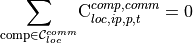
- declareComponentLinkedQuantityConstraints(pyM)[source]
Declare linked component quantity constraint, e.g. if an engine (E-Motor) is built also a storage (Battery) and a vehicle body (e.g. BEV Car) needs to be built. Not the capacity of the components, but the number of the components is linked.
- Parameters:
pyM (pyomo ConcreteModel) – a pyomo ConcreteModel instance which contains parameters, sets, variables, constraints and objective required for the optimization set up and solving.
- declareCommodityBalanceConstraints(pyM)[source]
Declare commodity balance constraints (one balance constraint for each commodity, location and time step)
- Parameters:
pyM (pyomo ConcreteModel) – a pyomo ConcreteModel instance which contains parameters, sets, variables, constraints and objective required for the optimization set up and solving.
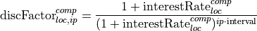
- declareObjective(pyM)[source]
Declare the objective function by obtaining the contributions to the objective function from all modeling classes. Currently, the only objective function which can be selected is the sum of the net present value of all components.

Objective Function detailed:

Contribution of design variable to the objective function

Contribution of binary design variables to the objective function

Contribution of operation variables to the objective function

With the annuity present value factor (Rentenbarwertfaktor):

and the discount factor.
- Parameters:
pyM (pyomo ConcreteModel) – a pyomo ConcreteModel instance which contains parameters, sets, variables, constraints and objective required for the optimization set up and solving.
- declareOptimizationProblem(timeSeriesAggregation=False, relaxIsBuiltBinary=False, relevanceThreshold=None)[source]
Declare the optimization problem belonging to the specified energy system for which a pyomo concrete model instance is built and filled with
basic time sets,
sets, variables and constraints contributed by the component modeling classes,
basic, component overreaching constraints, and
an objective function.
Default arguments:
- Parameters:
timeSeriesAggregation (boolean) –
states if the optimization of the energy system model should be done with
the full time series (False) or
clustered time series data (True).
* the default value is FalserelaxIsBuiltBinary – states if the optimization problem should be solved as a relaxed LP to get the lower bound of the problem.
* the default value is FalserelevanceThreshold (float (>=0) or None) – Force operation parameters to be 0 if values are below the relevance threshold.
* the default value is None
- optimize(declaresOptimizationProblem=True, relaxIsBuiltBinary=False, timeSeriesAggregation=False, logFileName='', threads=3, solver='None', timeLimit=None, optimizationSpecs='', warmstart=False, relevanceThreshold=None, includePerformanceSummary=False)[source]
Optimize the specified energy system for which a pyomo ConcreteModel instance is built or called upon. A pyomo instance is optimized with the specified inputs, and the optimization results are further processed.
Default arguments:
- Parameters:
declaresOptimizationProblem (boolean) –
states if the optimization problem should be declared (True) or not (False).
If true, the declareOptimizationProblem function is called and a pyomo ConcreteModel instance is built.
If false a previously declared pyomo ConcreteModel instance is used.
* the default value is TruerelaxIsBuiltBinary – states if the optimization problem should be solved as a relaxed LP to get the lower bound of the problem.
* the default value is FalsetimeSeriesAggregation (boolean) –
states if the optimization of the energy system model should be done with
the full time series (False) or
clustered time series data (True).
* the default value is Falsesegmentation (boolean) –
states if the optimization of the energy system model based on clustered time series data should be done with
aggregated typical periods with the original time step length (False) or
aggregated typical periods with further segmented time steps (True).
* the default value is FalselogFileName (string) – logFileName is used for naming the log file of the optimization solver output if gurobi is used as the optimization solver. If the logFileName is given as an absolute path (e.g. logFileName = os.path.join(os.getcwd(), ‘Results’, ‘logFileName.txt’)) the log file will be stored in the specified directory. Otherwise, it will be stored by default in the directory where the executing python script is called.
* the default value is ‘job’threads (positive integer) – number of computational threads used for solving the optimization (solver dependent input) if gurobi is used as the solver. A value of 0 results in using all available threads. If a value larger than the available number of threads are chosen, the value will reset to the maximum number of threads.
* the default value is 3solver (string) – specifies which solver should solve the optimization problem (which of course has to be installed on the machine on which the model is run).
* the default value is ‘gurobi’timeLimit (strictly positive integer or None) – if not specified as None, indicates the maximum solve time of the optimization problem in seconds (solver dependent input). The use of this parameter is suggested when running models in runtime restricted environments (such as clusters with job submission systems). If the runtime limitation is triggered before an optimal solution is available, the best solution obtained up until then (if available) is processed.
* the default value is NoneoptimizationSpecs (string) – specifies parameters for the optimization solver (see the respective solver documentation for more information). Example: ‘LogToConsole=1 OptimalityTol=1e-6’
* the default value is an empty string (‘’)warmstart (boolean) – specifies if a warm start of the optimization should be considered (not always supported by the solvers).
* the default value is FalserelevanceThreshold (float (>=0) or None) – Force operation parameters to be 0 if values are below the relevance threshold.
* the default value is NoneincludePerformanceSummary (boolean) – If True this will store a performance summary (in Dataframe format) as attribute (‘self.performanceSummary’) in the esM instance. The performance summary includes Data about RAM usage (assesed by the psutil package), Gurobi values (extracted from gurobi log with the gurobi-logtools package) and other various paramerts such as model buildtime, runtime and time series aggregation paramerters.
* the default value is False
Last edited: November 16, 2023
@author: FINE Developer Team (FZJ IEK-3)